Neural Network
Notes for Neural networks and deep learning
Artificial Neuron
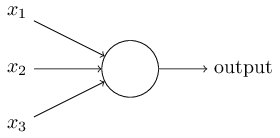
Perceptron
A perceptron takes several binary inputs, x1,x2,…x1,x2,…, and produces a single binary output:
Output = 0 if $\sum w_jx_j $ is not greater than threshold Output = 1 otherwise
bias, b = - threshold then Output = 0 if $w \cdot x + b$ is not greater than 0 Output = 1 otherwise
Sigmoid neuron
If a small change in some weight or bias only causes a coresponding small change in ouput, learning is possible. But a network of perceptrons can’t promise that. Thus sigmoid neuron is put forward.
Instead of being just 0 and 1, output of a sigmoid neuron is $\sigma(w\cdot x+b)$.
$\sigma(z)=\frac{1}{1+e^{-z}}$ is called activation function.
The Architecture of neural networks
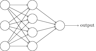
The leftmost layer - input layer
The rightmost layer - output layer
The middle layer - hidden layer
feedforward neural network - information is always fed forward, never fed back.
recurrent neural networks - in which neurons fire for some limited duration of time, before becoming quiescent.
Heuristic
Learning Algorithm - Gradient descent
cost function
It is also callde loss or objective function.Because $\Delta C = \frac{\partial C}{\partial v_1}\Delta v_1+\frac{\partial C}{\partial v_2}\Delta v_2$, we can make $\Delta v = -\eta \nabla C$,where $\eta$ is learning rate, to make C smaller.
Following are two typical cost functions:
- Quadratic cost function $C(w,b)=\frac{1}{2n}\sum ||y(x)-a||^2$
- Cross-entropy cost function $C = -\frac{1}{n} \sum_x \left[y \ln a + (1-y ) \ln (1-a) \right]$
Cross-entropy cost function is better than quadratic cost function because it avoids the problem of learning slowing down.
When $\sigma(z)=\frac{1}{1+e^{-z}}$, in a network blow
 we can obtain
\(\begin{align*}
\frac{\partial C}{\partial w_j} & = -\frac{1}{n} \sum_x \left(
\frac{y }{\sigma(z)} -\frac{(1-y)}{1-\sigma(z)} \right)
\frac{\partial \sigma}{\partial w_j} \\
& = -\frac{1}{n} \sum_x \left(
\frac{y}{\sigma(z)}
-\frac{(1-y)}{1-\sigma(z)} \right)\sigma'(z) x_j \\
& = \frac{1}{n}
\sum_x \frac{\sigma'(z) x_j}{\sigma(z) (1-\sigma(z))}
(\sigma(z)-y) \\
& = \frac{1}{n} \sum_x x_j(\sigma(z)-y)
\end{align*}\)
we can obtain
\(\begin{align*}
\frac{\partial C}{\partial w_j} & = -\frac{1}{n} \sum_x \left(
\frac{y }{\sigma(z)} -\frac{(1-y)}{1-\sigma(z)} \right)
\frac{\partial \sigma}{\partial w_j} \\
& = -\frac{1}{n} \sum_x \left(
\frac{y}{\sigma(z)}
-\frac{(1-y)}{1-\sigma(z)} \right)\sigma'(z) x_j \\
& = \frac{1}{n}
\sum_x \frac{\sigma'(z) x_j}{\sigma(z) (1-\sigma(z))}
(\sigma(z)-y) \\
& = \frac{1}{n} \sum_x x_j(\sigma(z)-y)
\end{align*}\)
since (\sigma’(z) = \sigma(z)(1-\sigma(z))).
Exception: When neurons in the final layer are linear neurons, the quadratic cost will not give rise to any problems with a learning slowdown since \(\begin{align*} \frac{\partial C}{\partial w^L_{jk}} & = \frac{1}{n} \sum_x a^{L-1}_k (a^L_j-y_j) \\ \frac{\partial C}{\partial b^L_{j}} & = \frac{1}{n} \sum_x (a^L_j-y_j) \end{align*}\)
Stochastic gradient descent
Due to the possible great number of variables, the computation of $\Delta C$ will take very long time.
So we can estimate $\Delta C = \frac{\sum \Delta C_x}{n} \approx \frac{\sum^m_{j=1} \Delta C_{X_j}}{m}$ . $X_1,X_2,…,X_j$ are refered as mini-batch.
After exhausting the training inputs by repeatedly training the network with different mini-batch, it is said to complete an epoch of training.
#Backpropagation There two assumptions we need about the cost function:
- The cost function can be written as an average $C = \frac{1}{n} \sum_x C_x $over cost functions $C_x$ for individual training examples, $x$.
- It can be written as a function of the outputs from the neural network.
Backpropagation is about understanding how changing the weights and biases in a network changes the cost function.
We define the error $\delta^l_j$ of neuron $j$ in layer $l$ by
$\delta^l_j=\frac{\partial C}{\partial z_j^l}$
Here comes the four fundamental equations behind backpropagation:

A Simple Handwritten Digits Classifier
It can be found in Github. Its typical usage(NumPy is required):
import network
import mnist_loader

training_data,validation_data,test_data = mnist_loader.load_data_wrapper()
net = network.Network([784, 30, 10])
net.SGD(training_data,30,10,3.0,test_data=test_data)